
Today we are happy to announce the general availability of RedisGraph v1.0. RedisGraph is a Redis module developed by Redis to add graph database functionality to Redis. We released RedisGraph in preview/beta mode over six months ago, and appreciate all of the great feedback and suggestions we’ve received from the community and our customers as we worked together on our first GA version.
Unlike existing graph database implementations, RedisGraph represents connected data as adjacency matrices instead of adjacency lists per data point. By representing the data as sparse matrices and employing the power of GraphBLAS (a highly optimized library for sparse matrix operations), RedisGraph delivers a fast and efficient way to store, manage and process graphs. In fact, our initial benchmarks are already finding that RedisGraph is six to 600 times faster than existing graph databases! Below, I’ll share how we’ve benchmarked RedisGraph v1.0, but if you’d like more information on how we use sparse matrices, check out these links in the meantime:
Before getting into our benchmark, I should point out that Redis is a single-threaded process by default. In RedisGraph 1.0, we didn’t release functionality to partition graphs over multiple shards, because having all data within a single shard allows us to execute faster queries while avoiding network overhead between shards. RedisGraph is bound to the single thread of Redis to support all incoming queries and includes a threadpool that takes a configurable number of threads at the module’s loading time to handle higher throughput. Each graph query is received by the main Redis thread, but calculated in one of the threads of the threadpool. This allows reads to scale and handle large throughput easily. Each query, at any given moment, only runs in one thread.

This differs from other graph database implementations, which typically execute each query on all available cores of the machine. We believe our approach is more suitable for real-time real-world use cases where high throughput and low latency under concurrent operations are more important than processing a single serialized request at a time.
While RedisGraph can execute multiple read queries concurrently, a write query that modifies the graph in any way (e.g. introducing new nodes or creating relationships and updating attributes) must be executed in complete isolation. RedisGraph enforces write/readers separation by using a read/write (R/W) lock so that either multiple readers can acquire the lock or just a single writer. As long as a writer is executing, no one can acquire the lock, and as long as there’s a reader executing, no writer can obtain the lock.
Now that we’ve set the stage with that important background, let’s get down to the details of our latest benchmark. In the graph database space, there are multiple benchmarking tools available. The most comprehensive one is LDBC graphalytics, but, for this release, we opted for a simpler benchmark released by TigerGraph in September 2018. It evaluated leading graph databases like TigerGraph, Neo4J, Amazon Neptune, JanusGraph and ArangoDB, and published the average execution time and overall running time of all queries on all platforms. The TigerGraph benchmark covers the following:
The TigerGraph benchmark reported TigerGraph to be 2-8000 times faster than any other graph database, so we decided to challenge this (well-documented) experiment and compare RedisGraph using the exact same setup. Since TigerGraph compared all other graph databases, we used the results published by their benchmark rather than repeating those tests.
Given that RedisGraph is v1.0 and we plan to add more features and functionalities in future release, for our current benchmark we decided to focus mainly on the k-hop neighborhood count query. Of course, we’ll publish results from other queries in the near future.
| Cloud Instance Type | vCPU | Mem (GiB) | Network | SSD |
|---|---|---|---|---|
| AWS r4.8xlarge | 32 | 244 | 10 Gigabit | EBS-Only |
| Name | Description and Source | Vertices | Edges |
|---|---|---|---|
| graph500 | Synthetic Kronecker graph http://graph500.org |
2.4 M | 64 M |
| Twitter user-follower directed graph http://an.kaist.ac.kr/traces/WWW2010.html | 41.6 M | 1.47 B |
The k-hop neighborhood query is a local type of graph query. It counts the number of nodes a single start node (seed) is connected to at a certain depth, and only counts nodes that are k-hops away.
Below is the Cypher code:
MATCH (n:Node)-[*$k]->(m) where n.id=$root return count(m)
Here, $root is the ID of the seed node from which we start exploring the graph, and $k represents the depth at which we count neighbors. To speed up execution, we used an index on the root node ID.
Although we followed the exact same benchmark as TigerGraph, we were surprised to see that they compared only a single request query response time. The benchmark failed to test throughput and latency under concurrent parallel load, something that is representative of almost any real-time real-world scenario. As I mentioned earlier, RedisGraph was built from the ground up for extremely high parallelism, with each query processed by a single thread that utilizes the GraphBLAS library for processing matrix operations with linear algebra. RedisGraph can than add threads and scale throughput in a close to linear manner.
To test the effect of these concurrent operations, we added parallel requests to the TigerGraph benchmark. Even though RedisGraph was utilizing just a single core, while other graph databases were using up to 32 cores, it achieved faster (and sometimes significantly faster) response times than any other graph database (with the exception of TigerGraph in the single request k-hop queries tests on the Twitter dataset).
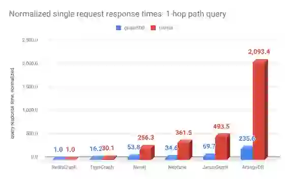
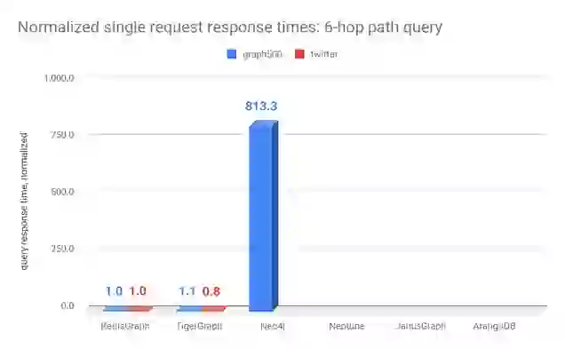
The single request benchmark tests are based on 300 seeds for the one and two-hop queries, and on 10 seeds for the three and six-hop queries. These seeds are executed sequentially on all graph databases. Row `time (msec)` represents the average response times of all the seeds per database for a given data set. Row ‘normalized’ per data set represents these average response times normalized to RedisGraph.
It is important to note that TigerGraph applied a timeout of three minutes for the one and two-hop queries and 2.5 hours for the three and six-hop queries for all requests on all databases (see TigerGraphs’s benchmark report for details on how many requests timed out for each database). If all requests for a given data set and given database timed out, we marked the result as ‘N/A’. When there is an average time presented, this only applies to successfully executed requests (seeds), meaning that the query didn’t time out or generate an out of memory exception. This sometimes skews the results, since certain databases were not able to respond to the harder queries, resulting in a better average single request time and giving a wrong impression of the database’s performance.In all the tests, RedisGraph never timed out or generated out of memory exceptions.
| Data set | Measure | RedisGraph | TigerGraph | Neo4j | Neptune | JanusGraph | ArangoDB |
|---|---|---|---|---|---|---|---|
| graph500 | time (msec) | 0.39 | 6.3 | 21.0 | 13.5 | 27.2 | 91.9 |
| normalized | 1 | 16.2 | 53.8 | 34.6 | 69.7 | 235.6 | |
| time (msec) | 0.8 | 24.1 | 205.0 | 289.2 | 394.8 | 1,674.7 | |
| normalized | 1 | 30.1 | 256.3 | 361.5 | 493.5 | 2,093.4 |
| Data set | Measure | RedisGraph | TigerGraph | Neo4j | Neptune1 | JanusGraph | ArangoDB2 |
|---|---|---|---|---|---|---|---|
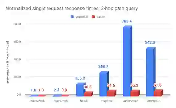
| graph500 | time (msec) | 30.7 | 71 | 4,180.0 | 8,250.0 | 24,050.0 | 16,650.0 |
| normalized | 1 | 2.3 | 136.2 | 268.7 | 783.4 | 542.3 | |
| time (msec) | 503.0 | 460.0 | 18,340.0 | 27,400.0 | 27,780.0 | 28,980.0 | |
| normalized | 1 | 0.9 | 36.5 | 54.5 | 55.2 | 57.6 |
| Data set | Measure | RedisGraph | TigerGraph | Neo4j | Neptune1 | JanusGraph | ArangoDB*2 |
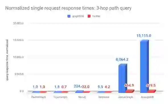
| graph500 | time (msec) | 229 | 410 | 51,380.0 | 2,270.0 | 1,846,710.0 | 3,461,340.0 |
| normalized | 1 | 1.8 | 224.4 | 9.9 | 8,064.2 | 15,115.0 | |
| time (msec) | 9301 | 6730 | 298,000.0 | 38,700.0 | 4,324,000.0 | 3,901,600.0 | |
| normalized | 1 | 0.7 | 32.0 | 4.2 | 464.9 | 419.5 |
| Data set | Measure | RedisGraph | TigerGraph | Neo4j | Neptune1 | JanusGraph | ArangoDB2 |
|---|---|---|---|---|---|---|---|
| graph500 | time (msec) | 1614 | 1780 | 1,312,700.0 | N/A | N/A | N/A |
| normalized | 1 | 1.1 | 813.3 | N/A | N/A | N/A | |
| time (msec) | 78730 | 63000 | N/A | N/A | N/A | N/A | |
| normalized | 1 | 0.8 | N/A | N/A | N/A | N/A |
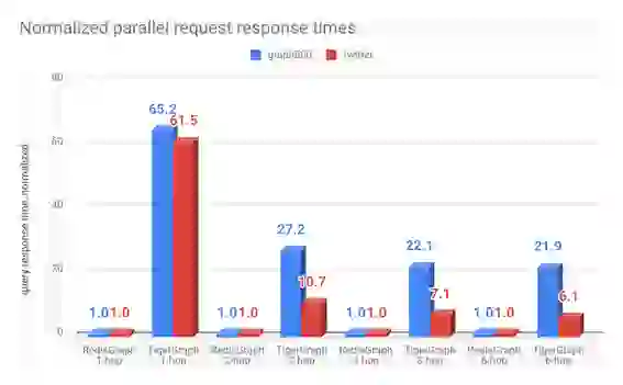
For the parallel requests test, we only compared RedisGraph and TigerGraph. This setup included 22 client threads running on the same test machine, which generated 300 requests in total. The results below show how long (in msec) it took for each graph database to answer all the requests combined, at each depth (one, two, three and six-hops).
For TigerGraph, we extrapolated results by multiplying the average response times of the single request times by 300, for each depth. We believe this is the best case scenario, since TigerGraph was already fully consuming all 32 cores for the single requests. Next time, we will repeat these test with TigerGraph under the same load of 22 clients and we expect (given the laws of parallelism and the overhead this will generate for executing parallel requests) our results will be even better.
| One-hop | Two-hop | Three-hop | Six-hop | ||||||
|---|---|---|---|---|---|---|---|---|---|
| Data set | Measure | RediGraph | Tiger | RedisGraph | Tiger | RedisGraph | Tiger | RedisGraph | Tiger |
| graph500 | time (msec) | 29 | 1,890 | 772 | 21,000 | 5,554 | 123,000 | 24,388 | 534,000 |
| normalized | 1 | 65.2 | 1 | 27.2 | 1 | 22.1 | 1 | 21.9 | |
| time (msec) | 117 | 7,200 | 12,923 | 138,000 | 286,018 | 2,019,000 | 3,117,964 | 18,900,000 | |
| normalized | 1 | 61.5 | 1 | 10.7 | 1 | 7.1 | 1 | 6.1 | |
We are very proud of these preliminary benchmark results for our v1.0 GA release. RedisGraph was started just two years ago by Roi Lipman (our own graph expert) during a hackathon at Redis. Originally, the module used a hexastore implementation but over time we saw way more potential in the sparse matrix approach and the usage of GraphBlas. We now have formal validation for this decision and RedisGraph has matured into a solid graph database that shows performance improvements under load of 6 to 60 times faster than existing graph solutions for a large dataset (twitter) and 20 to 65 times faster on a normal data set (graph500).
On top of that, RedisGraph outperforms Neo4j, Neptune, JanusGraph and ArangoDB on a single request response time with improvements 36 to 15,000 times faster. We achieved 2X and 0.8X faster single request response times compared to TigerGraph, which uses all 32 cores to process the single request compared to RedisGraph which uses only a single core. It’s also important to note that none of our queries timed out on the large data set, and none of them created out of memory exceptions.
During these tests, our engineers also profiled RedisGraph and found some low-hanging fruit that will make our performance even better. Amongst other things, our upcoming roadmap includes:
Happy graphing!
RedisGraph Team
January 17, 2019
After we published these RedisGraph benchmarking results, the folks at TigerGraph replied with some thoughts. While we appreciate hearing our competition’s perspective, we’d like to address their accusation of fake news. Read our benchmark update blog here.