 Stop testing, start deploying your AI apps. See how with MIT Technology Review’s latest research.
Download now


To benchmark the performance of our newly released RedisTimeSeries 1.2 module, we used the Time Series Benchmark Suite (TSBS). A collection of Go programs based on the work made public by InfluxDB and TimescaleDB, TSBS is designed to let developers generate datasets and then benchmark read and write performance. TSBS supports many other time-series databases, which makes it straightforward to compare databases.
For more on RedisTimeSeries 1.2, see RedisTimeSeries Version 1.2 Is Here!
This post will delve deep into the benchmarking process, but here’s the key thing to remember: RedisTimeSeries is fast…seriously fast! And that makes RedisTimeSeries by far the best option for working with time-series data in Redis:
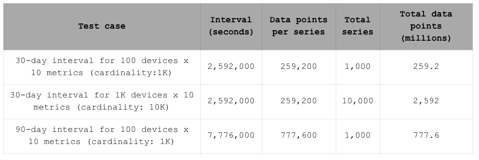
To compare RedisTimeSeries 1.2 with version 1.0.3, we choose three datasets: The first two have the same number of samples per time series but differ in cardinality.
Note: The maximum cardinality of a time-series dataset is defined as the maximum number of distinct elements that the dataset can contain or reference in any given point in time. For example, if a smart city has 100 Internet of Things (IoT) devices, each reporting 10 metrics (air temperature, Co2 level, etc.), spread across 50 geographical points, then the maximum cardinality of this dataset would be 50,000 [100 (deviceId) x 10 (metricId) x 50 (GeoLocationId)].
We chose these two datasets to benchmark query/ingestion performance versus the cardinality. The third dataset has the same cardinality as the first, but has three times as many samples in each time series. This dataset was used to benchmark the relationship between ingestion time and the number of samples in a time series.
The performance benchmarks were run on Amazon Web Services instances, provisioned through Redis’ benchmark testing infrastructure. Both the benchmarking client and database servers were running on separate c5.24xlarge instances. The database for these tests was running on a single machine with Redis Enterprise version 5.4.10-22 installed. The database consisted of 10 master shards.
In addition to these primary benchmark/performance analysis scenarios, we also enable running baseline benchmarks on network, memory, CPU, and I/O, in order to understand the underlying network and virtual machine characteristics. We represent our benchmarking infrastructure as code so that it is stable and easily reproducible.
The table below compares the throughput between the RedisTimeSeries version 1.0.3 and the new version 1.2 for all three datasets. You can see that the difference between the two versions is minimal. We did, however, introduce compression, which consumed 5% more additional CPU cycles. From this, we can conclude that if the shards are not CPU bound, then there is no throughput degradation by the compression.
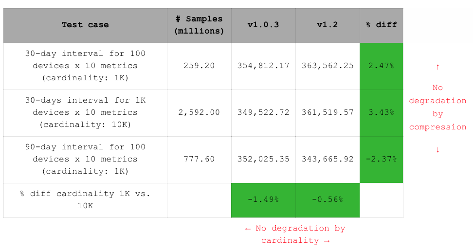
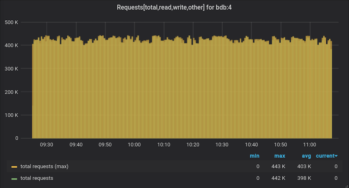
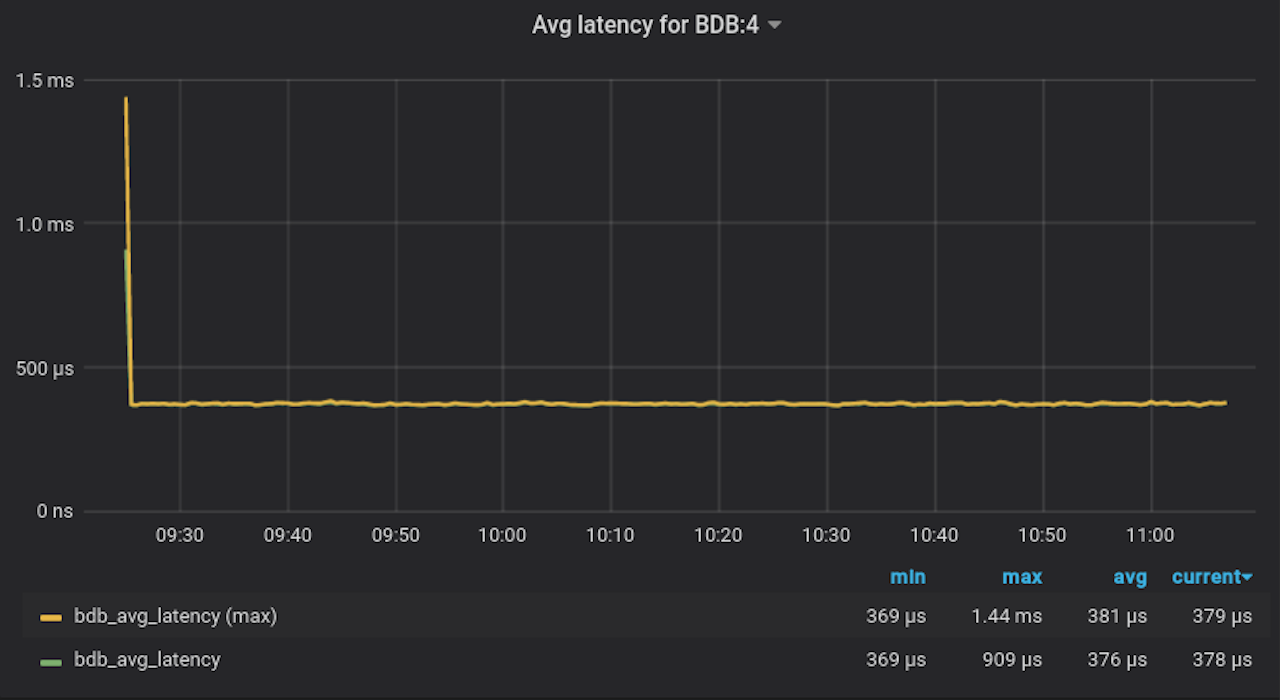
The three images below track throughput, latency, and memory consumption during the ingestion of the third (and largest) dataset. We inserted 800 million samples into a single database over the course of less than two hours. What is important here is that the latency and throughput do not degrade when there are more samples in a time series.The last row of the chart compares throughput over the first two datasets. There is almost no difference, which tells us that the performance does not degrade when the cardinality increases. Most other time-series databases degrade performance when the cardinality increases because of the underlying database and indexing technologies they use.

TSBS includes a range of different read queries. The charts below represent the query rate and query latency of multi-range queries comparing RedisTimeSeries version 1.0.3 to version 1.2. They show that query latency can improve up to 50% and throughput can increase up to 70%, depending on the query complexity, the number of accessed time series to calculate the response, and query time range. In general, the more complex the query, the more visible the performance gain.
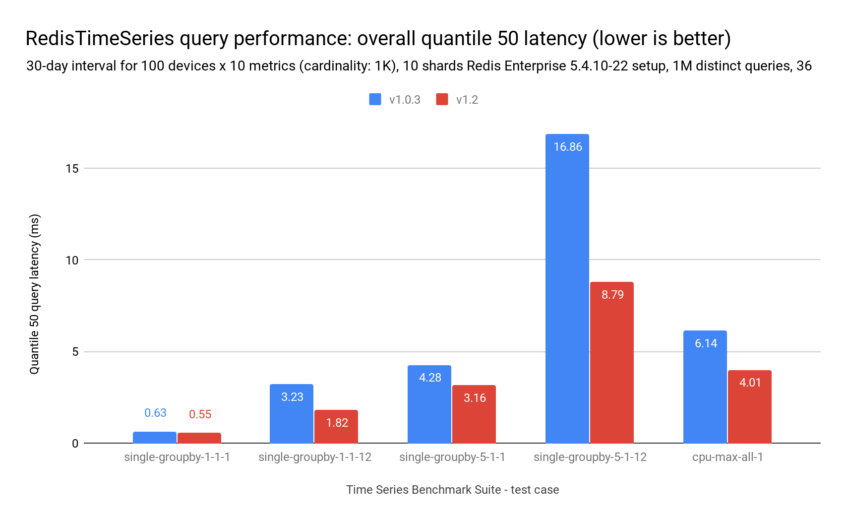
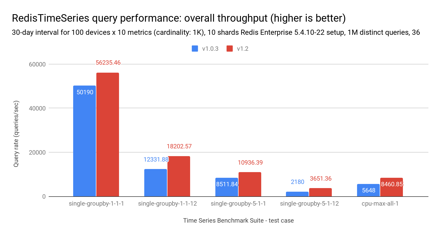
This behavior is due to both compression and changes to the API. Since more data fits in less memory space, fewer blocks of memory accesses are required to answer the same queries. Similarly, changes in the API’s default behavior of not returning the labels of each time series leads to substantial reductions in the load and overall CPU time on each TS.MRANGE command.
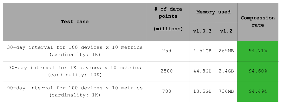
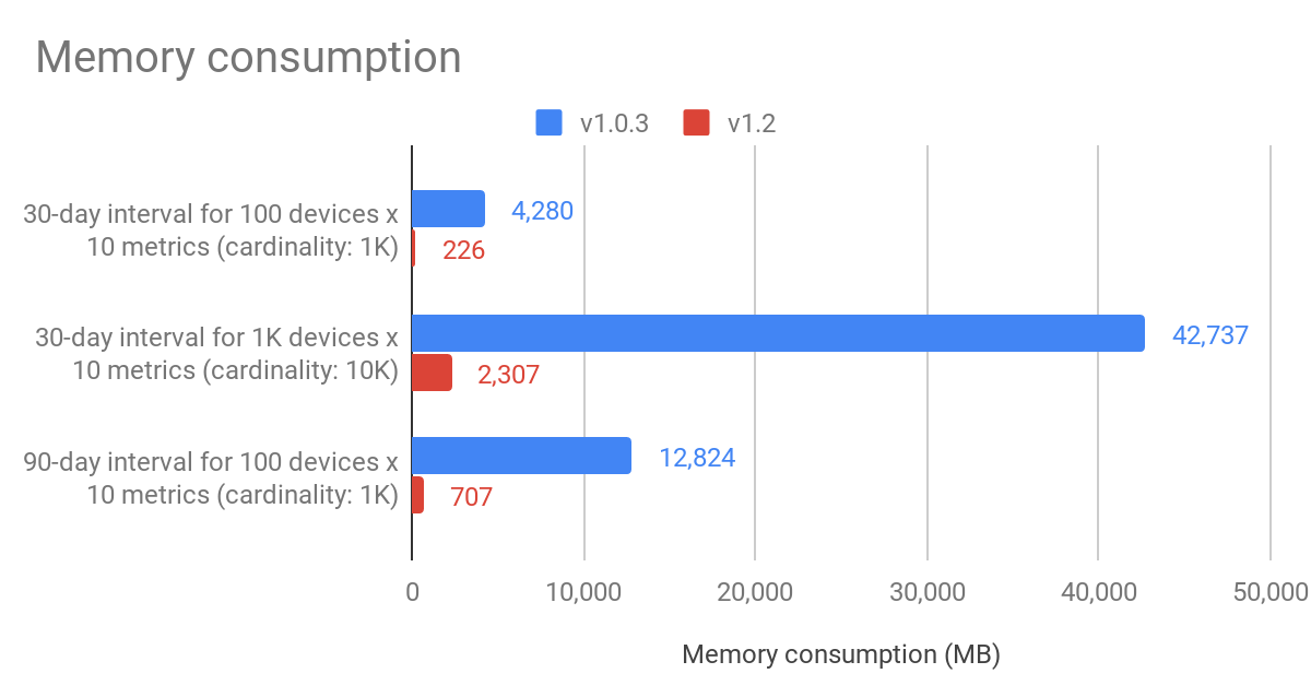
The addition of compression in RedisTimeSeries 1.2 makes it interesting to compare memory utilization in these three datasets. The result is a 94% reduction in memory consumption for all three datasets in this benchmark. Of course, this is a lab setup where timestamps are generated in fixed time intervals, which is ideal for double-delta compression (for more on double-delta compressions, see RedisTimeSeries Version 1.2 Is Here!). As noted, a memory reduction of 90% is common for real-world use cases.
RedisTimeSeries is seriously fast
When we launched RedisTimeSeries last summer, we benchmarked it against time-series modelling options with vanilla data structures in Redis, such as sorted sets and hashes or streams. In memory consumption, it already outperformed the other modeling techniques apart from Streams, which consumed half the memory that RedisTimeSeries did. With the introduction of Gorilla compression (more on that in this post: RedisTimeSeries Version 1.2 Is Here!), RedisTimeSeries is by far the best way to persist time series data in Redis.
In addition to demonstrating that there is no performance degradation by compression, the benchmark also showed there is no performance degradation by cardinality or by the number of samples in time series. The combination of all these characteristics is unique in the time-series database landscape. Add in the greatly improved read performance, and you’ll definitely want to check out RedisTimeSeries for yourself.
Finally, it’s important to note that the time-series benchmarking ecosystem is rich and community-driven—and we’re excited to be a part of it. Having a common ground for benchmarking has proven to be of extreme value in eliminating performance bottlenecks and hardening every solution in RedisTimeSeries 1.2. We have already started contributing to better understanding latency and application responsiveness on TSBS, and plan to propose further extensions to the current benchmarks.

